This tutorial will teach you how to freeze panes in Excel to keep them visible while scrolling from one region to another in your spreadsheet. When working with a large dataset, you may need to lock specific rows or columns to always keep them visible. You will learn how to freeze rows and columns in detail and what to do if the Freeze Panes option is disabled. Additionally, you will discover how to add the magic Freeze Panes command to your Quick Access Toolbar for easy access and quick freezing of your cells.
Freeze Rows in Excel
Freezing Rows in Excel is very easy to do with a few steps. To freeze rows in Excel, go to the View tab and click Freeze Panes in the Window group. You can freeze either the top row or multiple rows at once.
Go through the detailed guidelines below.
Freeze Top Row
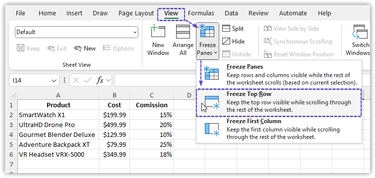
To freeze the first row in Excel, go to the View tab, click Freeze Panes from the Windows group, and click the Freeze Panes command.
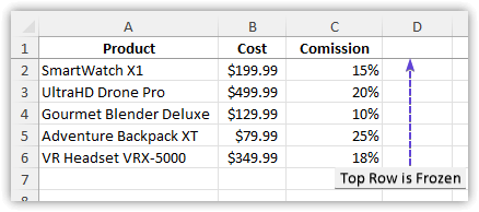
This will freeze the top row in your Excel worksheet. You can visualize the thin dark line indicating the top row is frozen. This will allow you to scroll down while keeping the first row in its position.
Freeze Multiple Rows
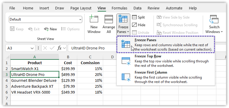
To freeze multiple rows, use the Freeze Panes command instead of the Freeze Top Row command.
For example, to freeze the first two rows of your spreadsheet, select the cell immediately below the second row. This selected cell must be the first cell at the beginning of the row. In other words, if you want to freeze the first two rows, select cell A3 and click the Freeze Panes command.
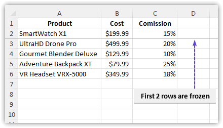
Therefore, you will see that the top two rows are frozen. Now, you can easily scroll down while keeping the first two rows in its position.
📓Notes: Microsoft Excel only allows you to freeze rows from the top. You cannot freeze rows from the middle of the sheet. You need to make sure that the rows you want to freeze are visible; otherwise, they will be hidden.
Freeze Columns in Excel
You can also freeze columns in Excel by using the Freeze Panes command.
Freeze First Column
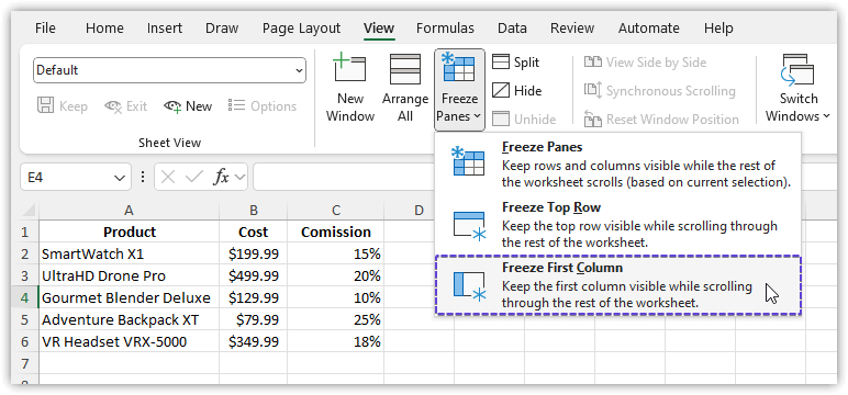
To lock the first column, click the View tab > Freeze Panes > Freeze First Column. This will lock the leftmost column of the worksheet while you scroll to the right.
Freeze Multiple Columns
Let’s say you want to freeze the first two columns in a sheet. You must select the top cell immediately to the right of the columns you want to lock.
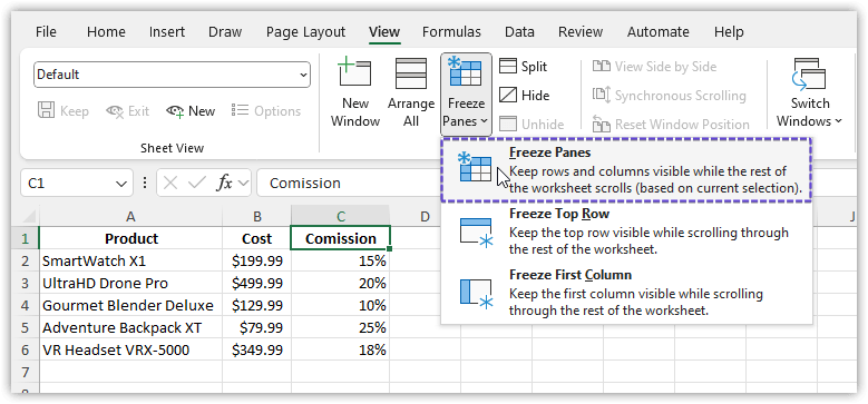
So, we will select cell C1 > then click View tab > Freeze Panes from Window group > Freeze Panes command.
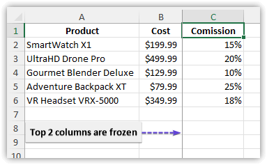
Therefore, you can see the spreadsheet is frozen up to column B.
📓Notes: Microsoft Excel only allows you to lock columns from the left. You cannot freeze columns from the middle of the sheet. You must ensure that the columns you want to lock are visible; otherwise, they will be hidden.
Freeze Rows and Columns in Excel
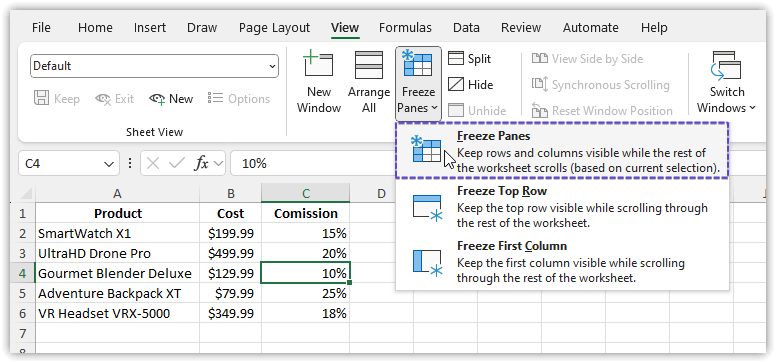
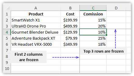
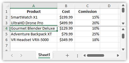
Aside from the option to lock rows and columns independently, you can also lock them both at the same time. Select a cell below the row and to the right of the column you want to lock. For example, select cell C4 to lock rows 1 to 3 and columns A to B.
As a result, you will visualize that the first two columns and the top three rows are locked simultaneously.
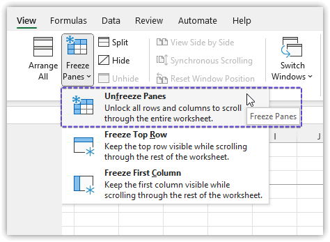
Unfreeze Rows and Columns in Excel
Click on the Unfreeze Panes command from the Windows group to unfreeze the frozen rows and columns.
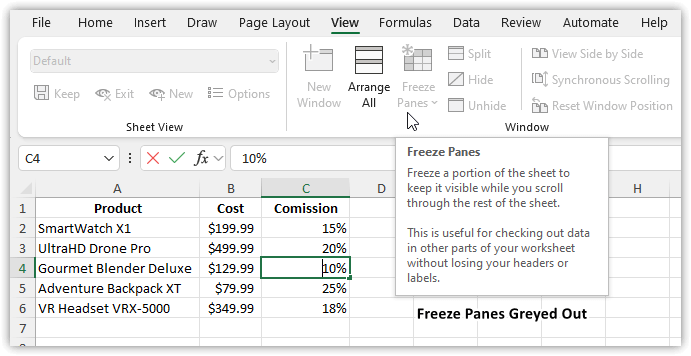
Freeze Panes not Working
You may find that the Freeze Panes command is disabled or greyed out. This could be due to two reasons:
- Your cell might be in Editing mode.
- Your worksheet might be protected.
Cell Is in Editing Mode
If your cell is in Editing mode, the Freeze Panes command will be greyed out. Press Enter or Esc to exit Editing mode.
Protected Worksheet
The Freeze Panes won't work in a protected sheet. So, unprotect the worksheet and try the Freeze Panes command again.
Other Ways to Lock Rows and Columns in Excel
Despite the use of freezing panes in Excel, you also have the option to split your worksheet into two or four sections.
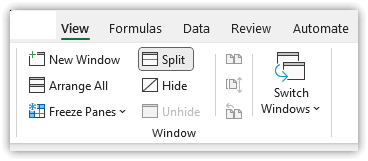
This feature enables you to scroll through each section independently. On the other hand, freezing panes allow you to lock specific rows and columns in place, making them visible while you scroll through the rest of the worksheet.
Add the Freeze Panes Button to the Quick Access Toolbar
You can easily add the Freeze Panes button in the Quick Access Toolbar. This will allow you to lock rows and columns with a single click.
- Click the down arrow at the top of the worksheet to expand the Customize Quick Access Toolbar options.
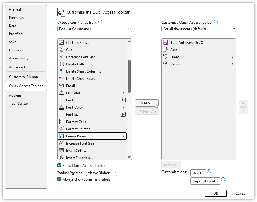
- Then, click on More Commands.
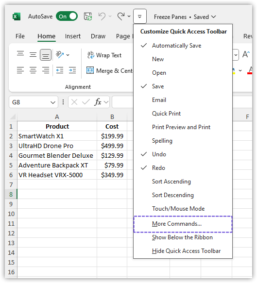
- Go serially by Choose Command from > Popular Commands > Freeze Panes > Add.
- Then, click OK.
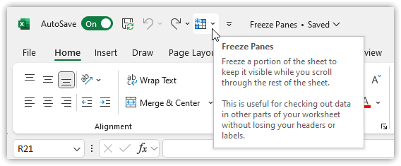
- As a result, the Freeze Panes button is added to the Quick Access Toolbar.
That’s how you will be able to freeze rows and columns separately or freeze both rows and columns simultaneously. You can unfreeze cells where it's not necessary. Additionally, you'll learn some reasons why the Freeze Panes feature might not work.